Fundamental Concepts

Cartesian Plane

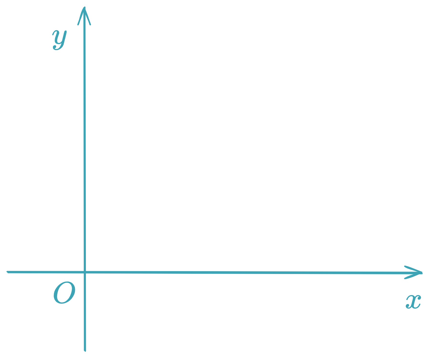
• Rectangular coordinate system: $x$-axis (abscissas) and $y$-axis (ordinates)
• Origin: point $(0,0)$

Quadrants

• Four quadrants labeled I to IV in counterclockwise order
• Signs:
  • Quadrant I: $(+,+)$
  • Quadrant II: $(-,+)$
  • Quadrant III: $(-,-)$
  • Quadrant IV: $(+,-)$

Points

• Representation: $P(x,y)$
  
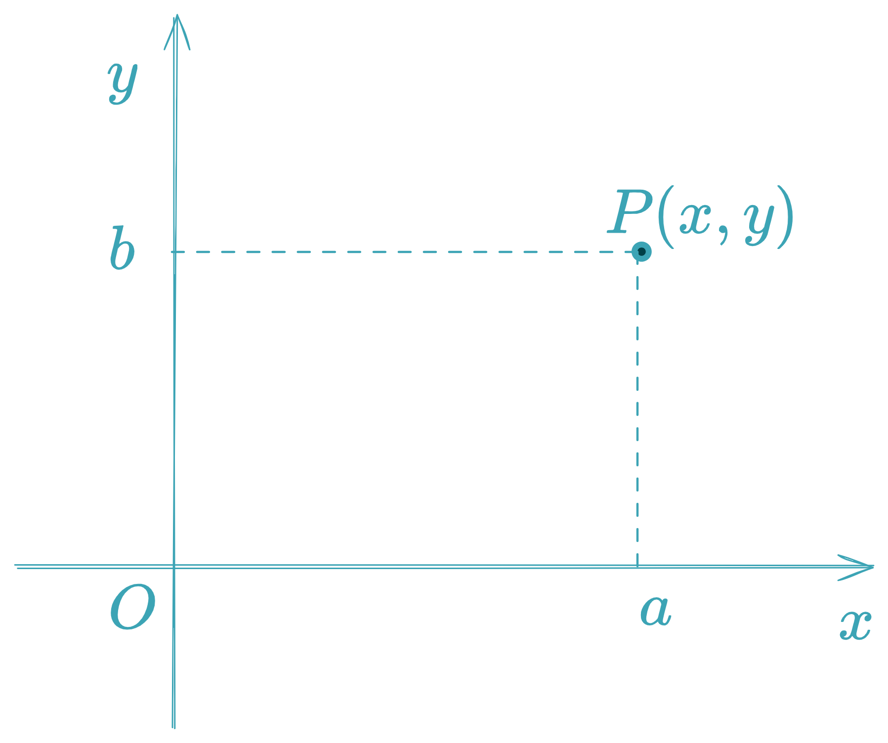
• Special points:
  • Origin: $O(0,0)$
  • On the $x$-axis: $(a,0)$
  • On the $y$-axis: $(0,b)$

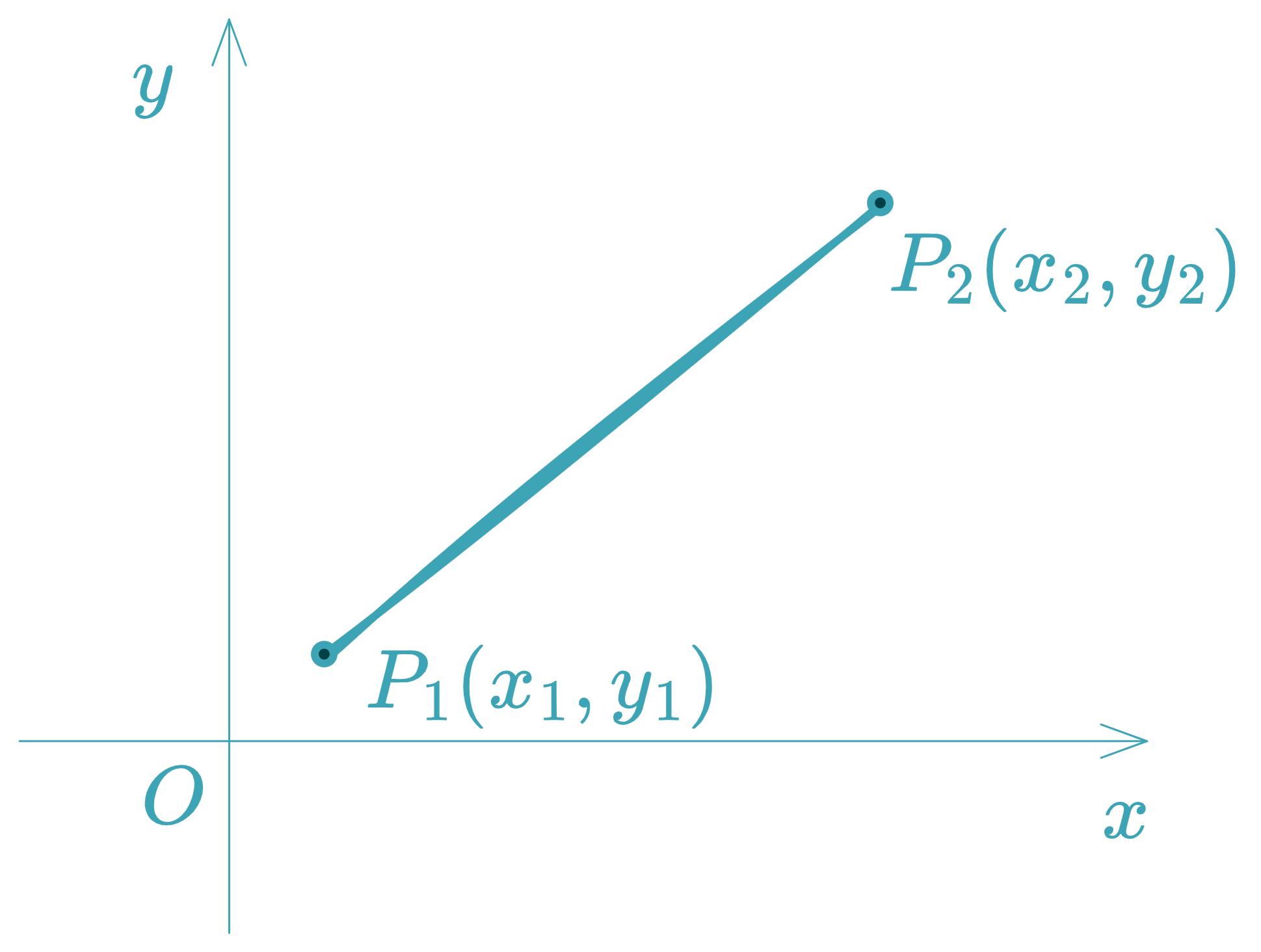
Distance Between Two Points

For $P_1(x_1,y_1)$ and $P_2(x_2,y_2)$:

$$d = \sqrt{(x_2 - x_1)^2 + (y_2 - y_1)^2}$$

Distance Between Two Points in Polar Coordinates

Given two points in polar coordinates:

• $P_1(r_1, \theta_1)$
• $P_2(r_2, \theta_2)$
  

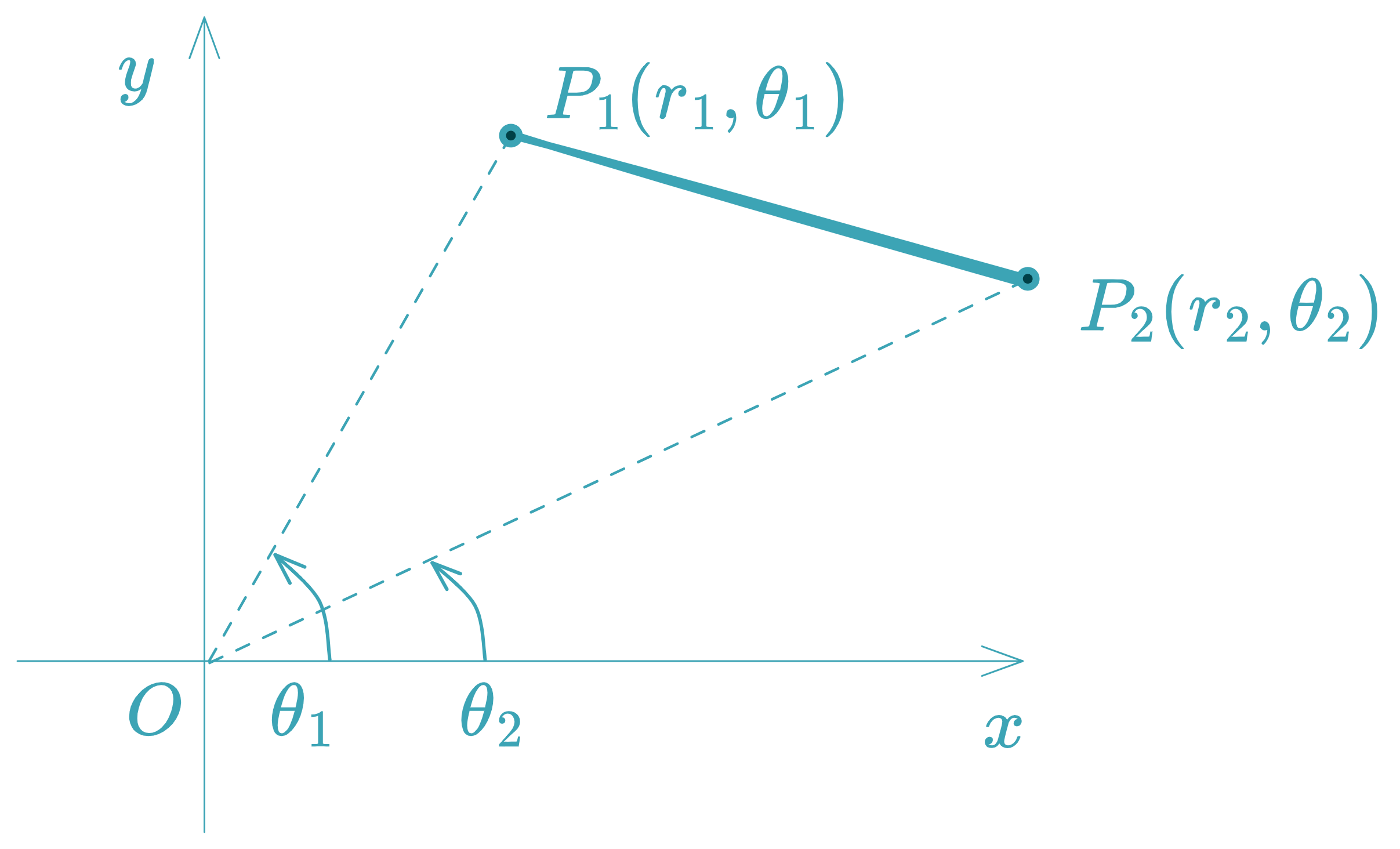
The distance $d$ between them is:

$$d = \sqrt{r_1^2 + r_2^2 - 2r_1r_2 \cos(\theta_2 - \theta_1)}$$

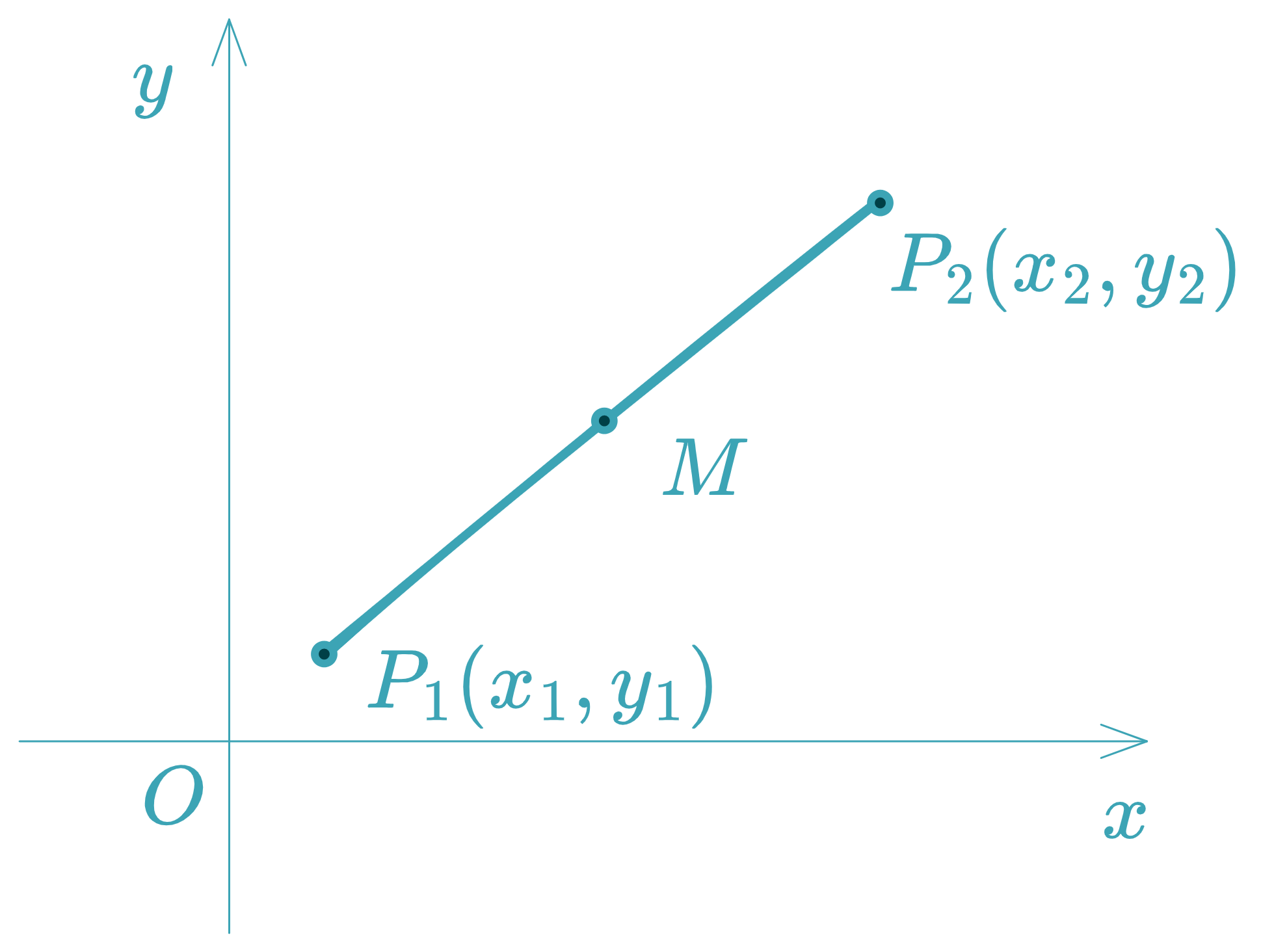
Midpoint

Midpoint $M$ between $P_1(x_1,y_1)$ and $P_2(x_2,y_2)$:

$$M\left(\frac{x_1+x_2}{2}, \frac{y_1+y_2}{2}\right)$$

Division of a Segment in a Given Ratio

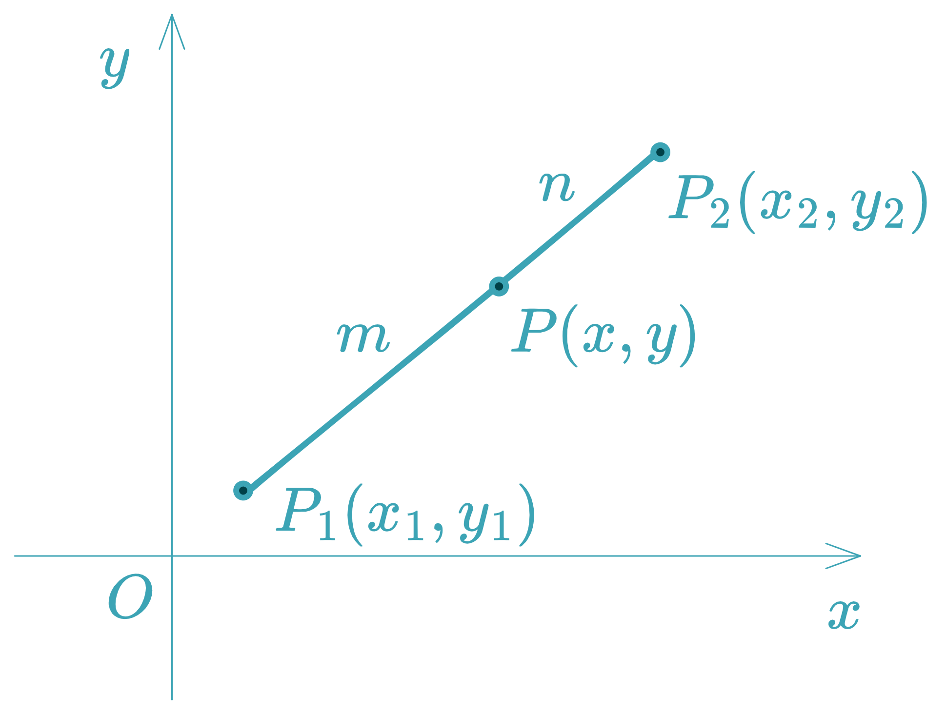
Point $P$ that divides segment $P_1P_2$ in the ratio $\frac{P_1P}{PP_2} = \frac{m}{n} = \lambda$:

$$x = \frac{nx_1 + mx_2}{n + m} = \frac{x_1 + \lambda x_2}{1 + \lambda}, \quad y = \frac{ny_1 + my_2}{n + m} = \frac{y_1 + \lambda y_2}{1 + \lambda}$$

$$P\left(\frac{x_1 + \lambda x_2}{1 + \lambda}, \frac{y_1 + \lambda y_2}{1 + \lambda}\right)$$

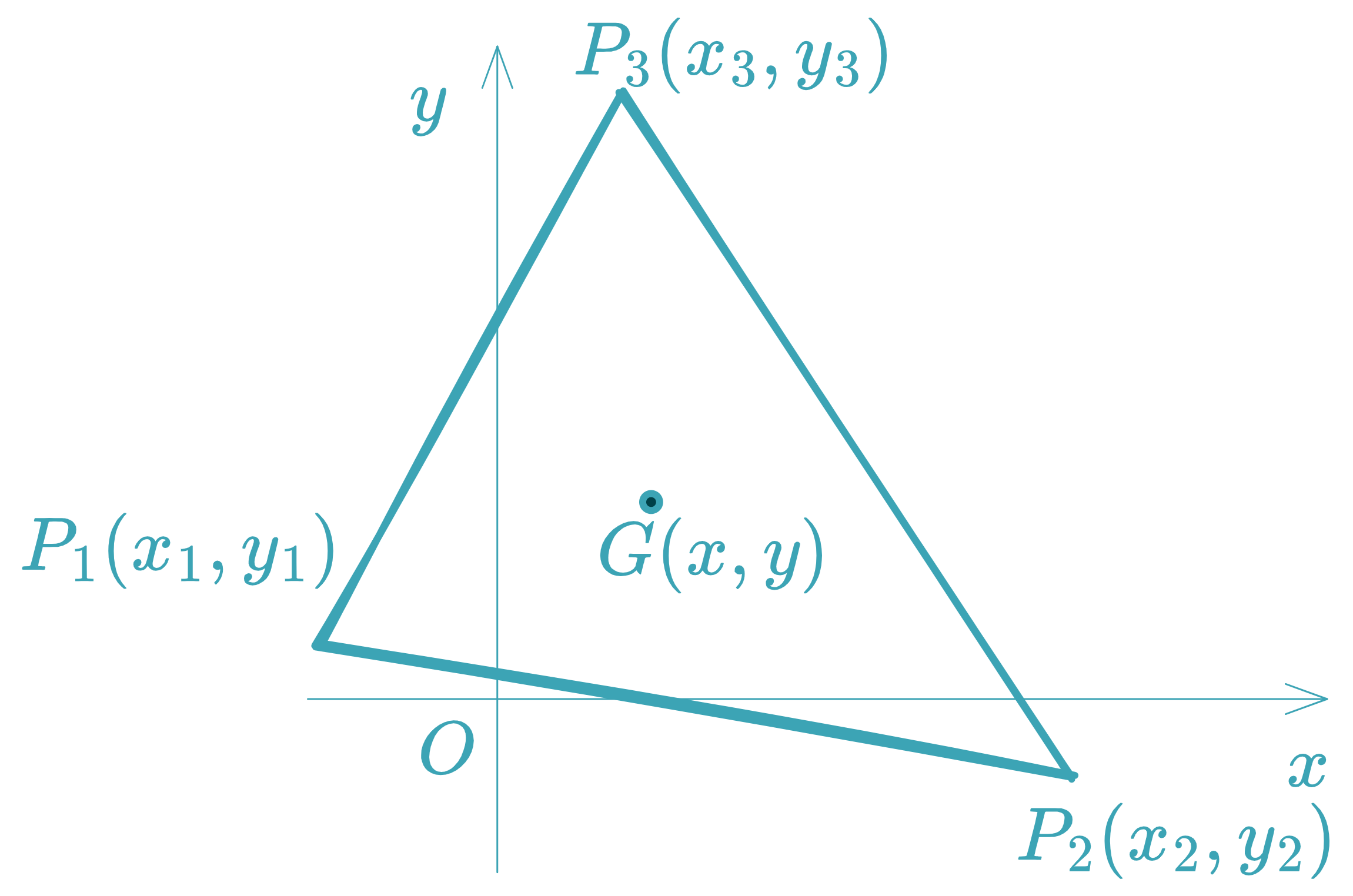
Coordinates of the Centroid of a Triangle

$$x = \frac{x_1 + x_2 + x_3}{3}$$

$$y = \frac{y_1 + y_2 + y_3}{3}$$

Area of a Triangle

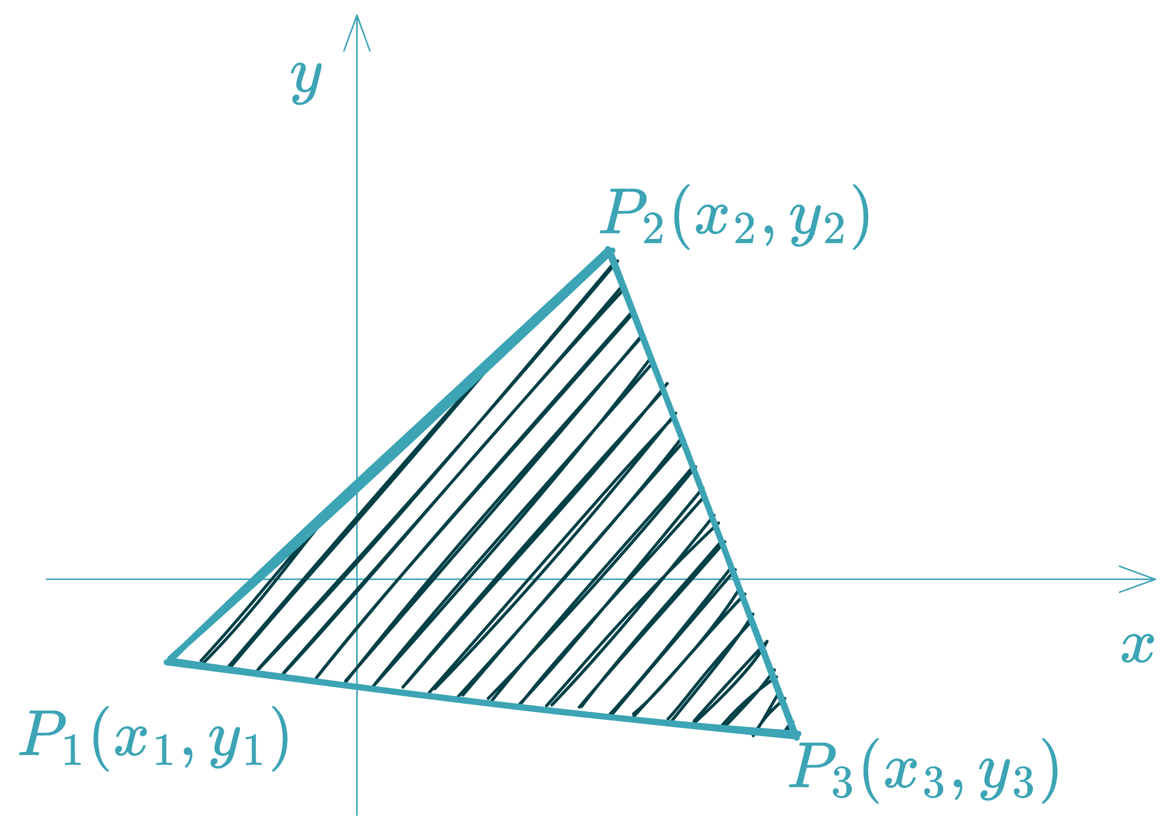
Given vertices $(x_1, y_1)$, $(x_2, y_2)$, and $(x_3, y_3)$, the area is:

$$\text{Area} = \frac{1}{2} \left| \begin{vmatrix} x_1 & y_1 & 1 \\ x_2 & y_2 & 1 \\ x_3 & y_3 & 1 \\ \end{vmatrix} \right|$$

Where the determinant evaluates to:

$$\begin{vmatrix} x_1 & y_1 & 1 \\ x_2 & y_2 & 1 \\ x_3 & y_3 & 1 \\ \end{vmatrix} = x_1(y_2 - y_3) - y_1(x_2 - x_3) + (x_2 y_3 - x_3 y_2)$$

In practice, this simplifies to:

$$\text{Area} = \frac{1}{2} \big| x_1(y_2 - y_3) + x_2(y_3 - y_1) + x_3(y_1 - y_2) \big|$$

title: Example  
Given vertices $P_1(2, 4)$, $P_2(5, 6)$, and $P_3(3, 1)$:  
1. **Form the matrix**:  
  $$ \begin{vmatrix}
   2 & 4 & 1 \\
   5 & 6 & 1 \\
   3 & 1 & 1 \\
   \end{vmatrix} $$

2. **Compute the determinant** (using Sarrus' rule):  
$$= 2(6 \cdot 1 - 1 \cdot 1) - 4(5 \cdot 1 - 3 \cdot 1) + 1(5 \cdot 1 - 3 \cdot 6)$$  
$$= 2(6 - 1) - 4(5 - 3) + 1(5 - 18)$$  
$$= 2(5) - 4(2) + 1(-13) = 10 - 8 - 13 = -11$$  
3. **Take absolute value and divide by 2**:  
$$\text{Area} = \frac{1}{2} |-11| = 5.5 \text{ units}^2$$  

Area of a Polygon

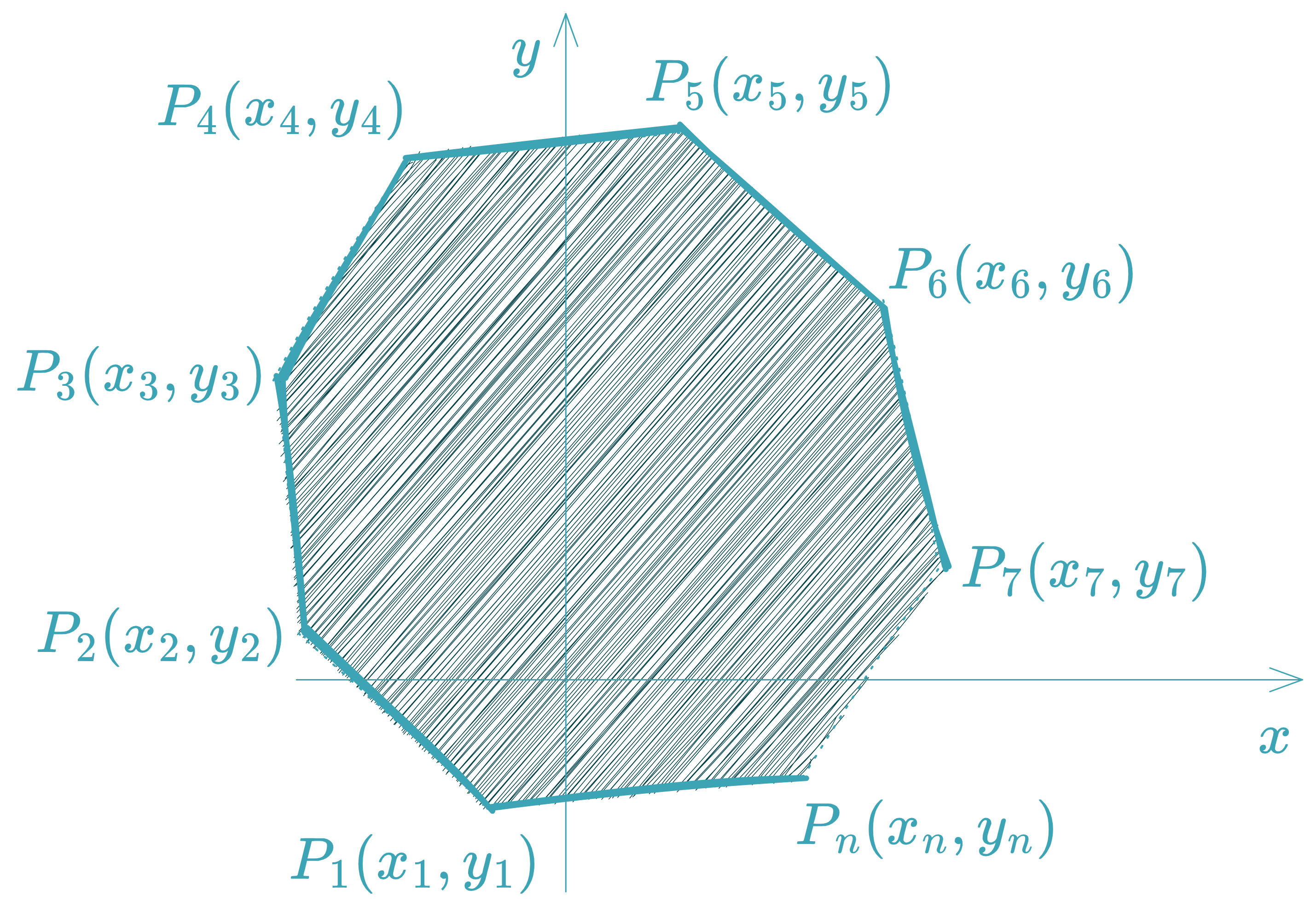
General Formula (Shoelace Formula)

For vertices $(x_1,y_1), (x_2,y_2), \ldots, (x_n,y_n)$:  
$$
\text{Area} = \frac{1}{2} \left| \sum_{i=1}^{n} \left( x_i y_{i+1} \right) - \sum_{i=1}^{n} \left( y_i x_{i+1} \right) \right|
$$  
where:  
- $x_{n+1} = x_1$ and $y_{n+1} = y_1$ (closes the polygon).  
- Vertices must be ordered **clockwise or counterclockwise** (no self-intersections).  

Steps to Apply the Formula:

1. Ordered list of vertices: Write coordinates in order (e.g., $P_1 \to P_2 \to P_3 \to \dots \to P_1$).
2. Sum 1 ($\Sigma_1$): Multiply each $x_i$ by the $y$ of the next vertex ($y_{i+1}$) and add them up.
3. Sum 2 ($\Sigma_2$): Multiply each $y_i$ by the $x$ of the next vertex ($x_{i+1}$) and add them up.
4. Subtract and take absolute value: Compute $|\Sigma_1 - \Sigma_2|$ and divide by 2.

title: Example  
Vertices in order: $P_{1}(2, 4)$, $P_{2}(5, 6)$, $P_{3}(3, 1)$, $P_{4}(1, 2)$.  
1. **Close the polygon by repeating $P_{1}$ at the end**:  
$$(2,4), (5,6), (3,1), (1,2), (2,4)$$  
2. **Compute $\Sigma_1$ (downward diagonals ➘)**:  
$(2 \times 6) + (5 \times 1) + (3 \times 2) + (1 \times 4) = 12 + 5 + 6 + 4 = 27$  
3. **Compute $\Sigma_2$ (upward diagonals ➚)**:  
$(4 \times 5) + (6 \times 3) + (1 \times 1) + (2 \times 2) = 20 + 18 + 1 + 4 = 43$  
4. **Area**:  
$$\text{Area} = \frac{1}{2} |27 - 43| = \frac{16}{2} = 8 \text{ units}^2$$  

Practice Problems

Level I

Level II

Level III